Learning from the Past - Time Series Predictions with Quantum Computing

A time series carries important information in the form of transition probabilities. For example, imagine we measure the ambient temperature on a daily basis. One day we measure a temperature of 17° C, and we want to know the probability that the temperature will be 19° C three days later. We refer to this quantity as the transition probability from 17 to 19 in 3 steps. More abstractly, given a natural number k and two data points i and j, we may ask what is the probability of transitioning from i to j in k steps (e.g., in k units of time). This quantity will be denoted T_ij(k). In our temperature example, i=17, j=19, and k=3.

Multidimensional time series, where multiple values are measured in time, may exhibit some additional interesting properties. For example, a two-dimensional time series could consist of two different stock prices as a function of time. In addition to the transition probabilities (exhibited for each time series individually), the two time series of stock prices may exhibit certain positive or negative correlations. Being able to identify and quantify connections between the values of different stocks can provide critical insights into their joint behaviour.

The last ingredient to motivate our work here is the concept of synthetic time series generation. For example, if a data scientist is unable to access sufficient data or sensitive time series data cannot be shared with them due to privacy issues, the data scientist might need synthetic time series in order to perform adequate analysis. Synthetic time series data should preserve properties from the original time series - including transition probabilities and multidimensional correlations - but should be different enough that they present as new time series.

Generative Adversarial Networks (GANs) and their quantum analog (qGANs) have previously fallen short of generating synthetic time series. Broadly speaking, modeling can range from generalized machine learning models which are broadly descriptive to deterministic learning models where computations can be carried out exactly. Deterministic models form the basis of physics and engineering, where the goal is to mathematically model various physical realities. For example, many exotic phenomena like black hole mergers (Zilhão et al. 2012) and RNA folding (Pincus et al. 2008) are modeled using various mathematical formalisms like algebraic tensor theories and stochastic equations. Development of these models often involves months, if not years, of effort and expertise in the relevant domain. And, more often than not, they fail to capture the intricate complexities of reality.

On the other hand, the explosive progress in computational resources has made it possible to train a computer to develop more and more sophisticated and expansive models. The last decade of machine learning research has shown the sheer success of models learned computationally from empirical data rather than developed analytically from underlying physical and mathematical principles. For example, at the time of writing this blog, no simple analytical model could pinpoint the exact position of a dog in a given image, while a neural network with reasonable computational power would take just minutes to do the same.

A considerable amount of work has been dedicated to bringing together learned and analytical models. This can be accomplished by either (a) bringing machine learning insights into the analytical model, or by (b) adding analytical constraints to the learned model. Both strategies have been successfully applied in various places. This is where quantum Hamiltonian learning methods kick in. More specifically, let's try to understand analytical and learning models in the case of time series data.

Given a time series, there exist a plethora of analytical modeling tools, from AutoRegressive Integrated Moving Average (ARIMA) models to Markov techniques (Bishop et al. 2007). On the learning side, one can pick a complete Deep Neural Network (DNN) to infer fundamental characteristics of a time series. A classic example of adding more analytical constraints into a learned time series model is the seminal work by Rumelhart et al. (1986), where the concept of Recurrent Neural Network (RNN) was first proposed. We introduce analytical constraints on a learning model based on quantum mechanics. Broadly, we want to constrain our learning space to a set of quantum Hamiltonians, or energy operators, that would closest replicate the characteristics of a given time series.

We start by translating the problem into quantum-friendly language. With adequate preprocessing, we can change each data point in the time series into basis state |i> for some i in {0,...,2^n-1} and an adequate n, or number of states into which our time series will be reduced. Now that we have our quantum time series, how can we obtain our transition probabilities? As the exact formalism is a bit technical, we may sacrifice some rigor for the sake of seeing the bigger picture (if you're not familiar with the terminology that follow, you may comfortably allow yourself to skip to the next paragraph).

The space where our data points - our quantum basis states - live is our system. For each particular unit of time, k, the k-step transition probabilities can be found via a quantum channel. Thanks to Stinespring's dilation theorem (Paulsen et al. 2003), each quantum channel can be obtained from a unitary operator acting on a larger space, consisting of both our original system and an additional "environment". By imposing further uniformity and coherence requirements on the underlying unitaries and environments, we find ourselves in a setting where a unitary acting on the system combined with the environment induces the transition probabilities of each individual time series in a multidimensional time series in a nice and uniform way. We refer to such series as K-Coherent, where K is the set of time steps in question.

So how do we achieve this goal? We construct a quantum circuit where the transition probabilities of the input time series are used in our training process to optimize the parameters of the circuit (Horowitz 2022). This eventually results in a unitary operator inducing transition probabilities that are close to the original values

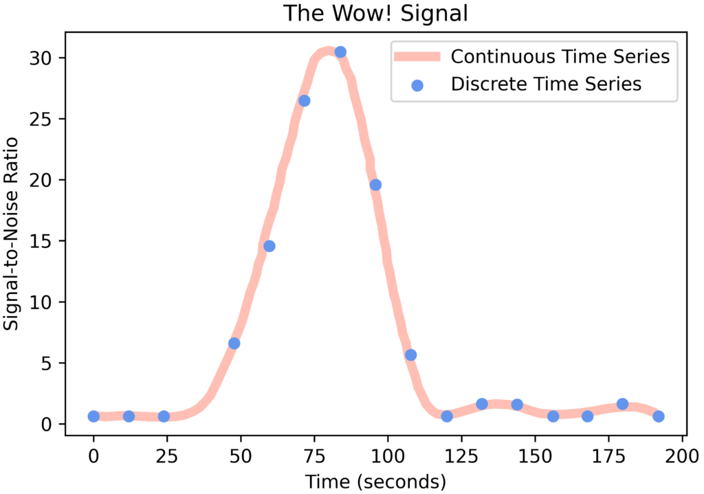
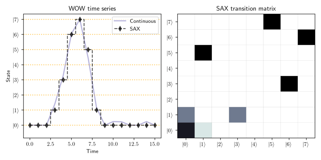
A key component of our learning process is the Symbolic Aggregate approXimation (SAX) algorithm. The SAX algorithm is commonly used in machine learning in order to reduce the size of time series data. An example of the SAX algorithm as applied to the Wow! Signal is shown in Figure 3. An input continuous time series (the violet curve in Figure 3) is reduced to a collection of discrete points (black diamonds in Figure 3), separable into quantum states (y-axis of Figure 3). In our quantum time series analysis, a continuous time series is reduced to two quantum states using the SAX algorithm.

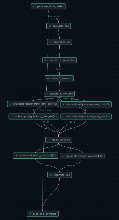
We assemble our algorithm using Covalent, our own open-source Pythonic workflow management tool. Covalent enables users to break their experiments down into manageable tasks that come together into a final workflow. The Covalent user interface allows users to visualize how each task fits into the workflow, as well as track the input and output of each task. Covalent tasks can be executed locally, on the cloud, a supercomputer, or a quantum computer. This makes it easy to construct quantum-hybrid experiments, where only specific tasks are run on quantum hardware. Using Covalent, our learning process can be broken down into discrete steps, where each step is created by defining a Python function with a Covalent electron decorator.

We used the following 9 functions in our learning process:

• Generate Time Series: A function to generate synthetic time series by solving a known stochastic differential equation
• Calculate δx_i: Calculating the first order difference series for having a stationary series
• Discretize 2^N: Using the Symbolic Aggregate approXimation (SAX) algorithm, we discretize the stationary series
• Find the Transition Probabilities T_ij(k): Calculating the transition matrix T_ij, the probability for i state to go j state in k time steps
• ⚛︎ Train Q Network: Iterative optimization requiring a quantum computer call to calculate the loss function and a classical computer call to run a minimization algorithm
• ⚛︎ Generate New δx_i Values: Using the trained network to generate new first order sequence by having quantum computer calls for each time step and repeating it multiple times
• Calculate Mean and Variance: Calculate the mean an standard deviation of first order difference at various time steps
• Calculate ∫δx_i → x_i: Integrate the first order difference to get back the original time series
• Plot and Compare: Plot the obtained time series along with the main time series

The steps with a ⚛︎ symbol are run on a quantum computer.

The Results

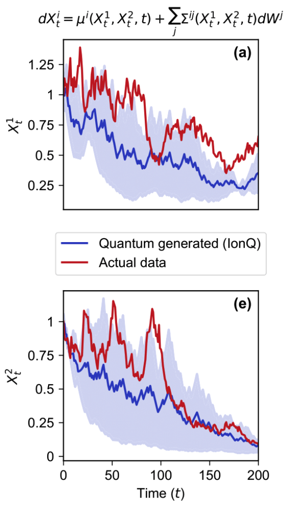
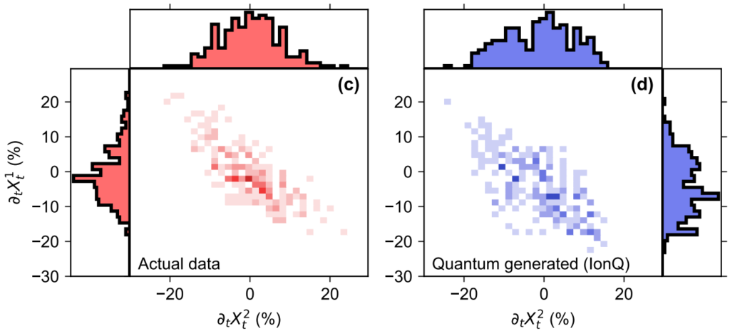
We ran our experiments on IonQ's 11-qubit trapped-ion quantum computer. Figure 5 shows both the input 2-dimensional time series data in red and the average quantum-generated time series plotted in blue. You can see that certain features, such as the negative slope, are preserved in the quantum-generated time series. In Figure 6, you can see that the correlation in the input time series data (plotted in red) and the correlation in the mean quantum-generated time series data (plotted in blue) are very similar.

The skeptical reader may rightly ask if we could have done the same thing using a classical computer. While we don't have proof that the answer is no, we do have some strong evidence suggesting that quantum computers might be particularly well-suited for such problems. We were able to show that finding a quantum process that generates the desired transition probabilities amounts to solving a rather complicated set of equations. In the most general case, this is known to be a computationally difficult task. Furthermore, we were able to experimentally observe that the process we learn exhibits a certain probabilistic property known as quantum non-Markovianity, which makes it very difficult to simulate using only a classical computer.

The Future

Our work opens the door to new intriguing directions of research. Can we find stronger evidence for quantum advantage? What are the limits of our algorithm? Does our algorithm work for all possible multidimensional time series? These questions remain wide open, and we invite the intrigued reader to help solve them.

References

[1] Christopher M. Bishop and Nasser M. Nasrabadi. Pattern Recognition and Machine Learning. Journal of Electronic Imaging, 16(4):049901, January 2007.

[2] Haim Horowitz, Pooja Rao, and Santosh Kumar Radha. A quantum generative model for multi-dimensional time series using hamiltonian learning. arXiv e-prints, page arXiv:2204.06150, April 2022.

[3] Vern Paulsen. Completely Bounded Maps and Operator Algebras. Cambridge Studies in Advanced Mathematics. Cambridge University Press, 2003.

[4] D. L. Pincus, S. S. Cho, C. Hyeon, and D. Thirumalai. Minimal models for proteins and RNA: From folding to function. arXiv e-prints, page arXiv:0808.3099, August 2008.

[5] David E. Rumelhart, Geoffrey E. Hinton, and Ronald J. Williams. Learning representations by back-propagating errors. , 323(6088):533–536, October 1986.

[6] Miguel Zilhão, Vitor Cardoso, Carlos Herdeiro, Luis Lehner, and Ulrich Sperhake. Collisions of charged black holes. ,85(12):124062, June 2012.